MS Excel Data Cleaning Tips

How to Reduce Size of Excel Files?

Did you ever wonder why your Excel File is so huge while it actually has very little information?

When you receive an excel file it was in KBs but when you make changes and save, file size surprisingly increased to MBs!!

Fortunately there are several ways to overcome this problem, this article will help you learn the Top Ten Awesome Tips & Tricks to Reduce Excel File Size to a great extent without losing the actual content.

Tip 1: Zip the Excel file

If you Don’t want to edit or make changes to your Excel File, but still want to reduce the file size? Then the best option will be Zip’ing the excel file, it will reduce upto 90% of file size depending upon the images and objects in the excel file.

Tip 2: Save the Excel file in .xlsb File Format

Do not want to edit anything in the spreadsheet (very similar to above case) only change is the file format in which you save the spreadsheet.

xlsb is Binary File Format, which will save your excel file in binary mode. Compressing/Reducing your Excel File Size to a great extent and the added advantage is, it can accommodate Macros unlike xlsx file format, and works way faster than any other excel file format.

Tip 3. Remove Unused Cells

Most people ignore this and burn their hand with huge file size and fatty lags.

What are these unused cells, basically there is a difference between ‘Actual Used Range’ and ‘Default Used Range’.

For example in the below given images, Actual data starts from cell ‘A1’ and lasts at cell ‘I14’ that is all we are interested in

But when I press CTRL+END key excel shows cell ‘I65526’ as the last used cell in my sheet. Surprising!! Yes it happens very often. The more beyond ‘Default Last Cell’ would be from ‘Actual Last Cell’, the more unnecessary size of excel workbook would it be having.

Do not worry just select the unused cells and delete the entire rows and save your file and see the change in file size.

Tip 4. Remove Cell Formatting

We do lot of formatting to the spreadsheet and we leave it there even though they are not adding any value to the main data. Removing formatting will save you more on file size, increase the spreadsheet performance and makes it look better or simple.

Follow below steps to remove formatting

1. Select the range which you do not need any kind of formatting.
2. Home Tab > Editing Group > Clear > Clear Formats

Best option if the spreadsheet contains lots of text.

Tip 5. Save the File in Right Version

Save your Excel file in the version that you are using. Saving your excel file in lower version will just make your file size increase. For example; if you are using Excel 2007 and above version, try to save your files in .xlsx, xlsm, .xlsb file formats unless otherwise the end user has the lower version.

Tip 6. Reduce the Size of Graphics

I Love Graphics in Spreadsheets, but not at the cost of pleasant spreadsheet performance, usability and presentability.

Remove Unnecessary Graphics as they take huge space.

Tip 7. Compress picture

Since picture take space and increases the file size, make sure you compress each picture in your spreadsheet.

Tip 8. Excessive use of Entire Column/Row Range in Formulas especially in Array formulas. I know how important and useful Array Formulas are, but try to use Array formulas as less as possible and lookout for alternative methods. As Array formulas will occupy for space and will slowdown spreadsheet performance.

Tip 9. Applying Conditional Formatting to ranges beyond the minimum needed to serve your purpose.

Tip 10. Employing more Query Tables: We do use query tables to get the data from external sources, but if you are done with the query table, better disconnect the table or just take the data and delete the query table as whole.

Here are the best possible ways to reduce the excel file size. What’s your way of choice in handling the excel file size. Leave your suggestions and questions in comments section below.

Note: Always make a backup of your original file before you try to compress it. While you’re trying out these tips, you could lose formatting, charts and other crucial components from your original workbook.

Courtesy to Raghu R

Microsoft Excel Functions

How to Provide Ranking ???

In this figure, products B & D are tied with sales of 87. The old RANK and RANK.EQ functions assign both of those products a rank of 2 and no product is ranked as 3.

Statisticians argue that products B & D should each receive a rank of 2.5, since the average of ranks 2 & 3 is 2.5. The new Excel 2010 function RANK.AVG will handle ties in this fashion.

Excel tricksters who use RANK to sort with a formula as described in the next topic want to make sure that every rank is used exactly once. They will use the formula shown in column G. This formula uses the original RANK function and then adds 1 if the ranked value is appearing a second time in the list.

=RANK($B2,$B$2:$B$8)+COUNTIF(B$2:B2,B2)-1

Courtesy By MrExcel.com

Excel FLOOR Function and CEILING Function

Excel has many great functions to allow you to round numbers but FLOOR and CEILING are two pretty cool ones.

While most functions allow you to round to a certain decimal place, these functions allow you to pick what you want to round to. If you need to round to large numbers like the nearest 100 or nearest 500, these functions can do it.

Let’s say we have these numbers below. We want to round the numbers in Column A to the nearest number in column B.

In row 2, we want to round 111 to the nearest 10.  What the FLOOR function will do is round it DOWN to the nearest 10.  The CEILING functions will round it UP to the nearest 10.

So the function would be:

We could also manually type the numbers in and use =FLOOR(111,10) and get the same result.  But references work just as well.

See how Excel takes 111 and rounds it down to the nearest 10 which is 110.

For the CEILING function we would use:

This works similar as FLOOR, except it rounds the number UP to the nearest 10 in this case.  So we get 120.

This will work to round for any instance.  You can round the the nearest 50, or 100 or 372.  It is up to you!  See below for our final results:

Courtesy By Joe.

REPLACE Function in Excel

REPLACE function in excel replaces a set of characters in a text string with a different set of characters, based on the number of characters specified.

At times, imported or copied data in an Excel spreadsheet carries unwanted characters or words, which can be replaced with good data using REPLACE function.

REPLACE function makes it easy to quickly rectify large amount of data. The function can be created for the first entry and then copied to all other cells, as done for most Excel functions.

REPLACE Function Example

Area code updation in phone number

REPLACE function can be used to update the first three digits in a phone number, on area code undergoing a change. In this example, Column C contains the new area code, Column D has the revised phone numbers.

REPLACE Function Syntax

The syntax for the REPLACE function is:

=REPLACE(old_text, start_num, num_chars, new_text)

Old_text – Text where some characters needs to be replaced. This can be a cell reference to the text.

Start_num - Mentions the start position (left to right) of the characters in old_text that needs to be replaced.

Num_chars - Mentions the number of characters to be replaced from the Start_num specified above.

New_text  – Text that will replace characters in old_text. This should be left blank if just unwanted characters need to be removed.

Text values that CONVERT Function accepts

Listed below are text values that CONVERT Function accepts for from_unit and to_unit (in quotation marks) :

WEIGHT AND MASS	FROM_UNIT / TO_UNIT
Gram	“g”
Slug	“sg”
Pound mass (avoirdupois)	“lbm”
U (atomic mass unit)	“u”
Ounce mass (avoirdupois)	“ozm”
TIME	FROM_UNIT / TO_UNIT
Year	“yr”
Day	“day”
Hour	“hr”
Minute	“mn”
Second	“sec”
DISTANCE	FROM_UNIT / TO_UNIT
Meter	“m”
Kilometer	“km”
Statute mile	“mi”
Nautical mile	“Nmi”
Inch	“in”
Foot	“ft”
Yard	“yd”
Angstrom	“ang”
Pica	“pica”
FORCE	FROM_UNIT / TO_UNIT
Newton	“N”
Dyne	“dyn” (or “dy”)
Pound force	“lbf”
TEMPERATURE	FROM_UNIT / TO_UNIT
Degree Celsius	“C” or “cel”
Degree Fahrenheit	“F” or “fah”
Kelvin	“K” or “kel”
LIQUID MEASURE	FROM_UNIT / TO_UNIT
Teaspoon	“tsp”
Tablespoon	“tbs”
Fluid ounce	“oz”
Cup	“cup”
U.S. pint	“pt” or “us_pt”
U.K. pint	“uk_pt”
Quart	“qt”
Gallon	“gal”
Liter	“l” or “lt”
PRESSURE	FROM_UNIT / TO_UNIT
Pascal	“Pa” or “p”
Atmosphere	“atm” or “at”
mm of Mercury	“mmHg”
ENERGY	FROM_UNIT / TO_UNIT
Joule	“J”
Erg	“e”
Thermodynamic calorie	“c”
IT calorie	“cal”
Electron volt	“eV” or “ev”
Horsepower-hour	“HPh” or “hh”
Watt-hour	“Wh” or “wh”
Foot-pound	“flb”
BTU	“BTU” or “btu”
POWER	FROM_UNIT / TO_UNIT
Horsepower	“HP” or “h”
Watt	“W” or “w”
MAGNETISM	FROM_UNIT / TO_UNIT
Tesla	“T”
Gauss	“ga”

CONVERT Function is used to convert data from one measurement unit to another.

For example, converting time from hours to minutes, distance from miles to kilometers, temperature from degrees Celsius to degrees Fahrenheit etc.

CONVERT Function Example

In this example, we’ll be converting table values from hours to minutes

=CONVERT(B3, “hr”, “mn”)

• Number      :   B3  ( Cell reference for the number to be converted)
• From_unit   :  “hr”  (Converted from unit – hours)
• To_unit       :  “mn” (Converted to unit – minutes)

CONVERT function result : 600 in cell C3

CONVERT Function Syntax

=CONVERT(number, from_unit, to_unit)

Number :   The value to be converted.

From_unit :   The measurement unit for Number.

To_unit :   The measurement unit for the converted value (result).

Value Function

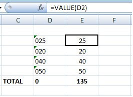
Excel mixes up data types at times and sees numerical data as text data. For eg. when you import data into Excel from another program / internet.

In such a situation, functions like SUM or AVERAGE lead to calculation errors.

VALUE Function converts numbers seen as Text to Values and make them function normally for SUM, AVERAGE and other numerical functions.

The syntax for the VALUE function is: = VALUE ( Text )

Text – Data to be converted. It can be actual data in quotation marks or a cell reference.

FIXED Function in Excel

Excel FIXED function returns number rounded to a specified number of decimal places as text. It uses commas as per specification.

SYNTAX

The syntax for the Microsoft Excel FIXED function is:

FIXED( number, [decimal_places], [no_commas] )

number is the number which has to be rounded.

decimal_places is optional. If ithis parameter is omitted, decimal places is assumed to be 2.

no_commas is optional. If set to TRUE, the result will not display commas. If set to FALSE, it will display commas in the result. If omitted, the result will display commas.

REPT Function in Excel

REPT(text, number_times) : Repeats text a given number of times. Use REPT to fill a cell with a number of instances of a text string.

Text - The text you want to repeat.
Number_times - The number of times to repeat text.

TRIM Function in Excel

TRIM(text) : Removes all spaces from a text string except for single spaces between words

Non Single Spaces

Courtesy By Systemfunda.com

Data Validation Tips

Data Validation a tool , through which Duplication of work can be avoided , Human errors can be minimised and TAT can be saved. There are many more rules. here a glimpse of the same.

Introduction: How do I set a maximum number for the cell?

1. Highlight the area you want to apply data validation to

2. You can highlight the entire column or click in the top cell, press Ctrl + Shift + Arrow down just to select pre-existing data.

3. Click on Data – Data Validation

4. On the Settings tab, choose Whole Number

5. Choose Less than or Less than or Equal to from the dropdown.

6. Enter the value e.g. 20 or if it’s a cell, click on the cell that contains the value you want to use as the maximum.

7. To help the users, it can be useful to add a message

8. Click on Input Message

9. In the Input Message box, type something like “number must be less than 20”

10. And if they persist….

11. Click on the Error Alert tab and in the Error Message box, you could type something like “what part of “enter a number less than 20 did you not understand?”

How do I only allow values between certain amounts ?

1. Follow steps 1-4 above

2. Choose Between from the dropdown

3. Enter your maximum and minimum values.

4. Apply the Input Message and Error Message as above if required. (Steps 7-11 from above)

How do I extend the data validation?

So your data validation is working well but now you find you need to extend it.

1. Highlight where you want to extend it to.

2. Make sure you have included cells with the data validation

3. Click on Data – Data Validation

4. You will receive a message that says “ The selection contains some cells without Data Validation settings. Do you want to extend Data Validation to these cells?”

5. Click on Yes

6. Your data validation dialog box will open up

7. Click OK.

How do I copy the data validation to another part of the sheet?

1. Click on cells with data validation

2. Click on Copy

3. Highlight the cells you want to copy the validation to.

4. Click on Paste – Paste Special.

5. Choose Validation

6. Now test.

How do I stop people changing some entries?

The most straightforward way to do that is by cell protection. But it’s not intuitive. The idea is that you indicate the areas you want people to be able to change and lock down everything else.

1. Begin by highlighting the areas you WANT people to be able to change.

2. Click Ctrl and 1 (to open the Formal Cells dialog box)

3. Click on the Protection tab

4. Clear the Locked box

5. Go to Review – Protect Sheet

6. Choose what you want people to be able to do.

7. Enter your password

8. You will then be prompted to re-enter it.

How do I only allow items from a specific list in?

The clue is in the name…you will be using a list

Method 1 – Create your list - static

1. Use this method if the items in your list will not be changing e.g. months, days etc.

2. On a separate worksheet, create the entries. (Type them vertically)

3. It can be useful to put your list entries on this sheet and call this sheet Lists

4. Highlight your list

5. In the Name Box (to left of formula bar) enter the name you want to give this range.

6. Note no spaces allowed in this name e.g. week_days NOT week days

7. Press Enter

8. Return to the sheet you want to apply the data validation to

9. Follow steps 1-3 in Introduction

10. Choose List from the list

11. Click in the Source box

12. Press F3 to call up your list of range names

13. Click on week_days

14. Now you will have a dropdown box where you can pick the week days from

15. Apply steps 7-11 from the Introduction if you want to add an error message.

Method 2 – Creating a dynamic list

1. Follow steps 1-3 as in Method 1

2. Click in your list.

3. Click Insert – Table

4. If your table doesn’t have a heading, leave the box for My table has headers unticked.

5. Note that it may add a “column 1” at the top.

6. You can remove that by deselecting Header Row from the Design tab (right hand side)

7. Now follow steps 5-15 from Method 1

8. The difference with this is that if you add a new item to your list, it will be automatically reflected in your data validation list

9. In order to make any changes other than the specified ones, you will have to unprotect the sheet (Review – Unprotect Sheet) by entering the password.

I want to delete the list

1. Click on Formulas – Name Manager

2. Click on the range you want to delete

3. Press Delete

I want to change the list

If you need to change the list

1. Simply follow the steps in Method 1 and at step 13, click on the new list you want to use.

How do I remove data validation?

1. Highlight the list you want to remove the data validation from

2. Choose Data – Data Validation

3. From the Allow box, choose Any Value

4. To extend the removal to all the cells, tick the Apply these changes to all other cells with the same settings box

I don’t even want other users to open my file.

1. Click on Review – Protect Workbook

2. Enter your password

3. Don’t forget to write down your password in a safe place

If you are responsible for the work of someone else, make sure they tell you what the password is. I’ve heard horror stories about disgruntled employees who have left without giving the password….(and on a side note, why don’t we call happy people gruntled…?)

OK, I’ll let them look, but not touch

1. Go to File – Save As

2. Click on Browse (if you are using Excel 2010 or later)

3. Go to folder you want to save it into.

4. Click on Tools (bottom right hand side)

5. Click General Options (nope, me neither )

6. Enter a password that allows the user to open or to modify.

7. Click OK and then Save.

I only want certain dates entered

From the Introduction, follow steps 1 – 3

1. On the Settings tab, choose Date

2. Note that from the Data tab, you can choose from any of the following:

3. Between (enter your Start Date and End Date)

4. Not Between ((enter your Start Date and End Date)

5. Equal to (enter your date here)

6. Not Equal To (Enter the date here)

7. Greater than (Enter the date here i.e. later than this date)

8. Less than (Enter the date here i.e. earlier than this date here)

9. Greater than or equal to (Enter the date here i.e. later than or equal to this date)

10. Less than or equal to (Enter the date here i.e. earlier than or equal this date here)

An example of how to use this would be to use =today() in the Date box using Less Than to restrict date entry to only those dates in the past.

I only want the users to enter certain text lengths in it.

An example of this would be where you only want users to be able to enter an 8 digit number.

1. Follow steps 1-3 from the Introduction

2. On the Settings tab, choose Text Length

3. Choose Equal to

4. Enter 8

5. Note that you have the same set of choices as referenced in the I only want certain dates entered section. i.e. greater than, lesser than etc.

6. Apply the Input Message and Error Message as above if required.

Prevention of Duplicate Entries:

It is set up by using the CountIf function.

Let’s say we want to prevent duplicates in cells M5:M100

1. From the Introduction follow steps 1-3

2. From the Allow box, choose Custom

3. In the Formula box enter the following: =COUNTIF($M$5:$M$100,M5)<=1

4. Note that what this function does is assess the range $M$5:$M$100 which is fixed. The M5 part of the formula will change as copied down. Therefore what it will do is see if what is in the current cell is counted more than once i.e. duplicate.

5. Apply your error messages if required (Introduction: steps 7-11)

I want the users to be able to sort and filter the list but not do ANYTHING ELSE.

One would think that specifying Sort and Autofilter in the Protect Sheet box would sort this. Nope, it doesn’t.

1. Highlight the area you want users to be able to sort and filter

2. Make sure the Filter is turned on (Data – Filter)

3. From Review – Allow users to Edit Ranges

4. Don’t use a password at this point

5. Click New

6. The range you have selected should appear in the dialog box

7. Click OK.

8. Then click Apply and OK

9. Now follow the instructions given in How do I stop people changing some entries?

10. Make sure the Sort and Autofilter boxes are ticked and that the Select Locked Cells and Select Unlocked Cells are deselected.

11. Note that for sorting you will have to use the Data – Sort dialog box to sort the data.

Courtesy By www. the-excel-expert.com

Microsoft Excel Worksheet and Workbook Limitations

CALCULATION SPECIFICATION & LIMITS

CHARTING SPECIFICATIONS & LIMITS

PIVOT TABLE AND PIVOT CHART REPORT LIMITATIONS

SHARED WORKBOOK SPECIFICATIONS AND LIMITS

Conditional Formatting Tips and Tricks

Finding the Unique Values with the help of Conditional Formatting.

Highlight mistakes, errors, omissions and repetitions

Entering large amounts of data into a spreadsheet is monotonous and pron to mistakes, omissions and repetitions. This can be avoided by using conditional formatting whenever typing or pasting a formula over a large range of cells.

To highlight a cell containing an error or omission:

Select “Conditional Formating”, “New Rule”, and “Format only cells that contain”

In the drop-down list under “Format only cells with:” select either “Error” or “Blanks” depending on what you want highlighted

Format your cells to your desired style

To highlight cells containing duplicate values:

Select “Conditional Formating”, “New Rule”, and “Format only unique or duplicate values”

Format your cells to your desired colors

Highlighting alternate rows or columns

Data presented in a large table is difficult to read because your eyes may have trouble following the rows and columns, especially when scrolling. To remedy this, try highlighting or changing the background color of alternative rows or columns. You could do this manually, but if you have a large table that keeps changing, you need to use Conditional Formatting.

Select the data section of your table you want to format

Click “Conditional formatting” in the “Home” ribbon

Click “New rule” near the bottom of the drop-down menu

Select “Use a formula to determine which cells to edit”

To highlight alternate rows, enter the formula =MOD(ROW(),2)=0 in the input box under “Format values where this formula is true:”

  This means whenever row() of the current cell is even, your desired formatting will be applied

•   To apply formatting to odd rows, just input =MOD(ROW(),2)=1 as the formula
•   To highlight alternate columns instead of rows, use =MOD(COLUMN(),2)=1 formula
•   What if you want to change background color of every 3rd row: use =MOD(ROW(),3)=0 instead

Format background colors, text, text color, borders, etc to your desired style. When you are done, the dialog should look something like the sample to the right:  Click OK.

Add “In-Cell” graphs

In-cell graphing is a handy trick that basically uses REPT() function, which repeats a character a given number of times, to generate bar-charts with in a cell. You can apply conditional formatting to the characters to give the charts good effect. Here is a sample:

 The graph highlights the cells that are greater than the average number of sales for the month by changing the font color to red and making it bold.

To create the graph:

Enter the formula =REPT(“I”,C4/100) in C4 of the “Graph” column then copy the formula to the cells beneath. (You will need to adjust the “divided by 100″ depending on the size of the number in the “Amount” column)

To create the conditional formating:

Click “Conditional Formating”, “New Rules” and “Use a formula to determine which cells to format”

Under “Format values where this formula is true:” enter

=($C4>AVERAGE($C$4:$C$33))

Click “Format” and change font color to “Red” and font style to “Bold” (or whatever format you want).

Click “Okay”

Creating a quick project plan / gantt chart using conditional formatting.

Project plans / gantt charts are everyday activity in most of our lives. Creating a simple and snazzy project plan template in excel is not a difficult job, using conditional formatting a bit of formulas you can do it no time.

First create a table structure like shown above, with columns like Activity, start and end day, day 1, 2,3, etc…

Now, whenever a day falls between start and end day for a corresponding activity, we need to highlight that row. For that we need to identify whether a day falls between start and end. We can do that with the below formulas,

    =IF(AND(F$8>=$D9, F$8<=$E9),"1","")

Which means, whenever, the day number represented on the top row is between start and end we will in 1 in the corresponding cell.

Next, whenever the cell value is 1, we will just fill the cell with a favorite color and change the font to same color, so that we dont see anything but a highlighted cell, better still, whenever you change the start or end dates, the color will change automatically. This will be done by conditional formatting like below:

Highlight the Non-Multiples

Shown below is the sample data for this conditional formatting example.

To add the conditional formatting, and highlight the non-multiples in column D:

• Select cells D2:D6, with D2 as the active cell

• On the Excel Ribbon's Home tab, click Conditional Formatting, and click New Rule

• In the New Formatting Rule dialog box, under 'Select a Rule Type', click 'Use a formula to determine which cells to format'

• In the formula box, type the MOD formula:   =MOD(D2,C2) <> 0

• Click Format, and on the Fill tab, select Red, then click OK, twice, to close the dialog boxes.

The MOD function returns the remainder after a number is divided by divisor. If the result is zero, then D2 is a multiple of C2.

Now the non-multiples in column D highlighted in red.

Format the Highest Value

To set up the conditional formatting for the highest value:

• Select cells C2:E6, with C2 as the active cell

• On the Excel Ribbon's Home tab, click Conditional Formatting, and click New Rule

• In the New Formatting Rule dialog box, under 'Select a Rule Type', click 'Use a formula to determine which cells to format'

• In the formula box, type the MAX formula:   =C2 = MAX($C2:$E2) The first reference to C2 is relative, so each cell will check its value compared to the MAX in the $C2:$E2 range.

• Click Format, and on the Font tab, select Red as the font colour, then click OK, twice, to close the dialog boxes.

Now the highest values are highlighted in each row.

Format the Second Highest Value

To set up the conditional formatting for the second highest value:

• Select cells C2:E6, with C2 as the active cell

• On the Excel Ribbon's Home tab, click Conditional Formatting, and click New Rule

• In the New Formatting Rule dialog box, under 'Select a Rule Type', click 'Use a formula to determine which cells to format'

• In the formula box, type the LARGE formula:   =C2 = LARGE($C2:$E2,2)

• Click Format, and on the Font tab, select Blue as the font colour, then click OK, twice, to close the dialog boxes.

Format the Lowest Value

To set up the conditional formatting for the second highest value:

• Select cells C2:E6, with C2 as the active cell

• On the Excel Ribbon's Home tab, click Conditional Formatting, and click New Rule

• In the New Formatting Rule dialog box, under 'Select a Rule Type', click 'Use a formula to determine which cells to format'

• In the formula box, type the MIN formula:   =C2 = MIN($C2:$E2)

• Click Format, and on the Font tab, select Green as the font colour, then click OK, twice, to close the dialog boxes.

Now the highest value in each row is highlighted in red, the second highest is blue, and the lowest is green.

Validation Rule for Conditional Formatting :

Conditional formatting won't let you refer to cells on a different worksheet, or in a different workbook. However, you can refer to a workbook level named range that's on a different worksheet.