How to Compare Two Columns in Excel and finding the even and odds

This is an interesting situation that often comes up. Namely, sometimes one needs to differentiate data in two different columns. There are so many processes in which Excel compare two lists and return differences. In this article, we will see the ways on how to compare two columns in Excel for differences.

Introduction

Here we have two lists where some fruits name is placed. We will compare the two lists for finding the differences. The two lists containing the fruits name is given below.

We will see 4 different processes of finding the differences between two columns. In every process, we will use the same table.

Compare Two Columns in Excel For Differences using Conditional Formatting

We can use the conditional formatting to highlight the unique values of two columns. The procedure is simple and given below.

• First, select the ranges where you want to apply the conditional formatting. In this example, the range is A2:B8

• Now, in the Home Tab click on to the Conditional Formatting and Under Highlight Cells Rules click on to Duplicate Values.

• In the Duplicate values Dialogue Box if you select Duplicate you will see the duplicate values of the two cells.

• If you select Unique in the Duplicate values Dialogue Box you will see the unique values of the two cells.

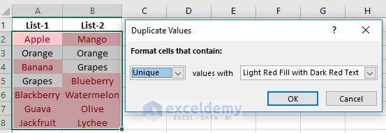
• Press OK to confirm the conditional formatting.

Compare Two Columns in Excel Using VLOOKUP

We can use the VLOOKUP function in Excel to find the differences between two lists or columns. The procedure is given below.

• In Cell C2 use the formula 

  Source code

  =IF(ISNA(VLOOKUP(A2,$B$2:$B$8,1,0)),"NO","YES")

  and press Enter.

• After pressing Enter, you will see the statement NO in cell C2. That is because the fruit name Apple from List-1 is not available in List-2.

• Now drag down the formulated cell downwards from C2 to C8 to see the differences between List-1 and List-2.

Compare Two Columns in Excel & Returns the Difference

Here we will be using IF, ISERROR, and MATCH functions to compare two columns. We will compare List-1 with List-2. The formula will calculate the two lists and will return the fruits name which is only in List-1. The procedure is given below.

• In Cell C2, write the formula 

  Source code

  =IF((ISERROR(MATCH(A2,$B$2:$B$14,0))),A2,"")

  and press enter.

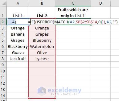
• After pressing Enter you will see the name of the fruit Apple which is only placed in List-1.

• Now drag down this formulated cell to see the fruits name which is only in List-1.

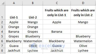
• In this same way, you can find the fruits name which is only in List-2. In that case, the formula will be,

  Source code

  =IF((ISERROR(MATCH(B2,$A$2:$A$15,0))),B2,"")

   which will be written in cell D2 and should be dragged down to find the comparison between two lists.

How to Compare Two Columns in Excel For Differences Using Formula

In this procedure, if List-1 contains any fruits name which is not placed in List-2, the formula that we will be using will say that the fruit name from List-1 is not found in List-2. Let`s start the comparison.

• In cell C2 write the formula

  Source code

  =IF(COUNTIF($B$2:$B$8, $A2)=0, "Not Found in List-2", "")

   and press enter.

• After pressing Enter you will see the statement, Not Found in List-2 has appeared. It is because the fruit name Apple from List-1 is not in List-2.

• Now, drag down the formulated cell C2 downwards to copy this formula for the rest of the cells of column C. By doing this, you will see the differences between the two columns.

Courtesy By: www.exceldemy.com

Hidden Facts about Microsoft

Hidden Facts about Microsoft

Total number of characters that a cell can contain 32,767 characters
Hyperlinks in a worksheet 66,530 hyperlinks
Undo levels 100
Smallest allowed positive number 2.2251E-308
Largest allowed positive number 9.99999999999999E+307
Dependency on a single cell 4 billion formulas that can depend on a single cell
Latest date allowed for calculation December 31, 9999
Largest amount of time that can be entered 9999:59:59

Office has been downloaded 340 million times on Iphones, Ipads and Android devices.

Skype Users make upto 3 billion minutes of calls each day .

Outlook.com has more than 400 million active users.

Every excel sheet has 17,179,869,184 cells.

If you need 1 second to fill out 1 cell, it would take you 545 years to complete the whole worksheet.

It is not possible to Name a worksheet “History” in Excel.

There are more than 500 keyboard shortcuts in MS Excel.

Microsoft donates an average of $2.6 million in software each day to more than 86,000 nonprofits around the world.

More than 1.2 billion people use Microsoft office in 140 countries and 107 languages around the world.

MS Excel Data Cleaning Tips

How to Reduce Size of Excel Files?

Did you ever wonder why your Excel File is so huge while it actually has very little information?

When you receive an excel file it was in KBs but when you make changes and save, file size surprisingly increased to MBs!!

Fortunately there are several ways to overcome this problem, this article will help you learn the Top Ten Awesome Tips & Tricks to Reduce Excel File Size to a great extent without losing the actual content.

Tip 1: Zip the Excel file

If you Don’t want to edit or make changes to your Excel File, but still want to reduce the file size? Then the best option will be Zip’ing the excel file, it will reduce upto 90% of file size depending upon the images and objects in the excel file.

Tip 2: Save the Excel file in .xlsb File Format

Do not want to edit anything in the spreadsheet (very similar to above case) only change is the file format in which you save the spreadsheet.

xlsb is Binary File Format, which will save your excel file in binary mode. Compressing/Reducing your Excel File Size to a great extent and the added advantage is, it can accommodate Macros unlike xlsx file format, and works way faster than any other excel file format.

Tip 3. Remove Unused Cells

Most people ignore this and burn their hand with huge file size and fatty lags.

What are these unused cells, basically there is a difference between ‘Actual Used Range’ and ‘Default Used Range’.

For example in the below given images, Actual data starts from cell ‘A1’ and lasts at cell ‘I14’ that is all we are interested in

But when I press CTRL+END key excel shows cell ‘I65526’ as the last used cell in my sheet. Surprising!! Yes it happens very often. The more beyond ‘Default Last Cell’ would be from ‘Actual Last Cell’, the more unnecessary size of excel workbook would it be having.

Do not worry just select the unused cells and delete the entire rows and save your file and see the change in file size.

Tip 4. Remove Cell Formatting

We do lot of formatting to the spreadsheet and we leave it there even though they are not adding any value to the main data. Removing formatting will save you more on file size, increase the spreadsheet performance and makes it look better or simple.

Follow below steps to remove formatting

1. Select the range which you do not need any kind of formatting.
2. Home Tab > Editing Group > Clear > Clear Formats

Best option if the spreadsheet contains lots of text.

Tip 5. Save the File in Right Version

Save your Excel file in the version that you are using. Saving your excel file in lower version will just make your file size increase. For example; if you are using Excel 2007 and above version, try to save your files in .xlsx, xlsm, .xlsb file formats unless otherwise the end user has the lower version.

Tip 6. Reduce the Size of Graphics

I Love Graphics in Spreadsheets, but not at the cost of pleasant spreadsheet performance, usability and presentability.

Remove Unnecessary Graphics as they take huge space.

Tip 7. Compress picture

Since picture take space and increases the file size, make sure you compress each picture in your spreadsheet.

Tip 8. Excessive use of Entire Column/Row Range in Formulas especially in Array formulas. I know how important and useful Array Formulas are, but try to use Array formulas as less as possible and lookout for alternative methods. As Array formulas will occupy for space and will slowdown spreadsheet performance.

Tip 9. Applying Conditional Formatting to ranges beyond the minimum needed to serve your purpose.

Tip 10. Employing more Query Tables: We do use query tables to get the data from external sources, but if you are done with the query table, better disconnect the table or just take the data and delete the query table as whole.

Here are the best possible ways to reduce the excel file size. What’s your way of choice in handling the excel file size. Leave your suggestions and questions in comments section below.

Note: Always make a backup of your original file before you try to compress it. While you’re trying out these tips, you could lose formatting, charts and other crucial components from your original workbook.

Courtesy to Raghu R

Microsoft Excel Functions

How to Provide Ranking ???

In this figure, products B & D are tied with sales of 87. The old RANK and RANK.EQ functions assign both of those products a rank of 2 and no product is ranked as 3.

Statisticians argue that products B & D should each receive a rank of 2.5, since the average of ranks 2 & 3 is 2.5. The new Excel 2010 function RANK.AVG will handle ties in this fashion.

Excel tricksters who use RANK to sort with a formula as described in the next topic want to make sure that every rank is used exactly once. They will use the formula shown in column G. This formula uses the original RANK function and then adds 1 if the ranked value is appearing a second time in the list.

=RANK($B2,$B$2:$B$8)+COUNTIF(B$2:B2,B2)-1

Courtesy By MrExcel.com

Excel FLOOR Function and CEILING Function

Excel has many great functions to allow you to round numbers but FLOOR and CEILING are two pretty cool ones.

While most functions allow you to round to a certain decimal place, these functions allow you to pick what you want to round to. If you need to round to large numbers like the nearest 100 or nearest 500, these functions can do it.

Let’s say we have these numbers below. We want to round the numbers in Column A to the nearest number in column B.

In row 2, we want to round 111 to the nearest 10.  What the FLOOR function will do is round it DOWN to the nearest 10.  The CEILING functions will round it UP to the nearest 10.

So the function would be:

We could also manually type the numbers in and use =FLOOR(111,10) and get the same result.  But references work just as well.

See how Excel takes 111 and rounds it down to the nearest 10 which is 110.

For the CEILING function we would use:

This works similar as FLOOR, except it rounds the number UP to the nearest 10 in this case.  So we get 120.

This will work to round for any instance.  You can round the the nearest 50, or 100 or 372.  It is up to you!  See below for our final results:

Courtesy By Joe.

REPLACE Function in Excel

REPLACE function in excel replaces a set of characters in a text string with a different set of characters, based on the number of characters specified.

At times, imported or copied data in an Excel spreadsheet carries unwanted characters or words, which can be replaced with good data using REPLACE function.

REPLACE function makes it easy to quickly rectify large amount of data. The function can be created for the first entry and then copied to all other cells, as done for most Excel functions.

REPLACE Function Example

Area code updation in phone number

REPLACE function can be used to update the first three digits in a phone number, on area code undergoing a change. In this example, Column C contains the new area code, Column D has the revised phone numbers.

REPLACE Function Syntax

The syntax for the REPLACE function is:

=REPLACE(old_text, start_num, num_chars, new_text)

Old_text – Text where some characters needs to be replaced. This can be a cell reference to the text.

Start_num - Mentions the start position (left to right) of the characters in old_text that needs to be replaced.

Num_chars - Mentions the number of characters to be replaced from the Start_num specified above.

New_text  – Text that will replace characters in old_text. This should be left blank if just unwanted characters need to be removed.

Text values that CONVERT Function accepts

Listed below are text values that CONVERT Function accepts for from_unit and to_unit (in quotation marks) :

WEIGHT AND MASS	FROM_UNIT / TO_UNIT
Gram	“g”
Slug	“sg”
Pound mass (avoirdupois)	“lbm”
U (atomic mass unit)	“u”
Ounce mass (avoirdupois)	“ozm”
TIME	FROM_UNIT / TO_UNIT
Year	“yr”
Day	“day”
Hour	“hr”
Minute	“mn”
Second	“sec”
DISTANCE	FROM_UNIT / TO_UNIT
Meter	“m”
Kilometer	“km”
Statute mile	“mi”
Nautical mile	“Nmi”
Inch	“in”
Foot	“ft”
Yard	“yd”
Angstrom	“ang”
Pica	“pica”
FORCE	FROM_UNIT / TO_UNIT
Newton	“N”
Dyne	“dyn” (or “dy”)
Pound force	“lbf”
TEMPERATURE	FROM_UNIT / TO_UNIT
Degree Celsius	“C” or “cel”
Degree Fahrenheit	“F” or “fah”
Kelvin	“K” or “kel”
LIQUID MEASURE	FROM_UNIT / TO_UNIT
Teaspoon	“tsp”
Tablespoon	“tbs”
Fluid ounce	“oz”
Cup	“cup”
U.S. pint	“pt” or “us_pt”
U.K. pint	“uk_pt”
Quart	“qt”
Gallon	“gal”
Liter	“l” or “lt”
PRESSURE	FROM_UNIT / TO_UNIT
Pascal	“Pa” or “p”
Atmosphere	“atm” or “at”
mm of Mercury	“mmHg”
ENERGY	FROM_UNIT / TO_UNIT
Joule	“J”
Erg	“e”
Thermodynamic calorie	“c”
IT calorie	“cal”
Electron volt	“eV” or “ev”
Horsepower-hour	“HPh” or “hh”
Watt-hour	“Wh” or “wh”
Foot-pound	“flb”
BTU	“BTU” or “btu”
POWER	FROM_UNIT / TO_UNIT
Horsepower	“HP” or “h”
Watt	“W” or “w”
MAGNETISM	FROM_UNIT / TO_UNIT
Tesla	“T”
Gauss	“ga”

CONVERT Function is used to convert data from one measurement unit to another.

For example, converting time from hours to minutes, distance from miles to kilometers, temperature from degrees Celsius to degrees Fahrenheit etc.

CONVERT Function Example

In this example, we’ll be converting table values from hours to minutes

=CONVERT(B3, “hr”, “mn”)

• Number      :   B3  ( Cell reference for the number to be converted)
• From_unit   :  “hr”  (Converted from unit – hours)
• To_unit       :  “mn” (Converted to unit – minutes)

CONVERT function result : 600 in cell C3

CONVERT Function Syntax

=CONVERT(number, from_unit, to_unit)

Number :   The value to be converted.

From_unit :   The measurement unit for Number.

To_unit :   The measurement unit for the converted value (result).

Value Function

Excel mixes up data types at times and sees numerical data as text data. For eg. when you import data into Excel from another program / internet.

In such a situation, functions like SUM or AVERAGE lead to calculation errors.

VALUE Function converts numbers seen as Text to Values and make them function normally for SUM, AVERAGE and other numerical functions.

The syntax for the VALUE function is: = VALUE ( Text )

Text – Data to be converted. It can be actual data in quotation marks or a cell reference.

FIXED Function in Excel

Excel FIXED function returns number rounded to a specified number of decimal places as text. It uses commas as per specification.

SYNTAX

The syntax for the Microsoft Excel FIXED function is:

FIXED( number, [decimal_places], [no_commas] )

number is the number which has to be rounded.

decimal_places is optional. If ithis parameter is omitted, decimal places is assumed to be 2.

no_commas is optional. If set to TRUE, the result will not display commas. If set to FALSE, it will display commas in the result. If omitted, the result will display commas.

REPT Function in Excel

REPT(text, number_times) : Repeats text a given number of times. Use REPT to fill a cell with a number of instances of a text string.

Text - The text you want to repeat.
Number_times - The number of times to repeat text.

TRIM Function in Excel

TRIM(text) : Removes all spaces from a text string except for single spaces between words

Non Single Spaces

Courtesy By Systemfunda.com